Survey weights help make survey estimates more representative of the target population. Many surveys also use complex sample designs involving stratification and clustering. These design features should be taken into account when estimating standard errors and confidence intervals.
This resource shows how to apply survey weights and account for survey design in R through examples using data from the 2017 British Social Attitudes Survey.
The examples show how to:
apply survey weights when calculating a mean.
specify a survey design using the survey package.
estimate means and proportions with confidence intervals.
produce estimates for population subgroups.
For an introduction to the concepts covered here, including survey weights, stratification, clustering and design variables, see the companion resource Survey Explainer: Survey weights and design variables.
You can use this resource as a simple reference, or follow the examples using your own copy of the data. Information on the required software and data is provided below.
2 Survey weighting and design in R
There are several ways to apply survey weights in R. A key distinction is between general weighting functions which apply weifhts without accounting for the survey design, and survey-specific approaches, which can account for survey design when estimating measures of precision such as confidence intervals.
2.1General weighting functions
Base R provides some functionality for weighted analysis, including functions such as weighted.mean() and regression models like lm() that allow the use of weights. Additional R packages offer convenient functions for calculating weighted estimates. For example, the Hmisc package includes functions such as wtd.mean(), wtd.var(), and wtd.quantile(), while the summarytools package supports weighted frequency tables and common descriptive statistics.
2.2Survey analysis functions
The functions discussed above can be used for producing weighted estimates, but they do not allow users to fully account for survey design features such as stratification, clustering and unequal selection probabilities.
The survey package provides a set of functions that apply survey weights and correctly account for the sample design when estimating standard errors and confidence intervals. Before using the package, you must identify the survey weights and design variables and create a survey design object. This resource includes step-by-step examples showing how to do this.
The srvyr package is based on the survey package and designed to work better with dplyr and the tidyverse approach to R including piping.
3 Data and software requirements
To work through the examples on your own machine, you will need:
basic familiarity with R.
an up-to-date copy of R.
the dplyr, haven, survey, Hmisc and ggplot2 packages.
a UK Data Service account (for downloading the data)
From the information in the dataset user guide, we can see that the 2017 British Social Attitudes (BSA) survey used a three-stage stratified random sample.
Postcode sectors were selected first, followed by addresses and then individuals.
The primary sampling units (postcode sectors) were:
first stratified by sub-region, population density, and the proportion of owner-occupied housing.
selected with probability proportional to size, so postcode sectors containing more addresses had a greater chance of being selected.
To account for this design in the analysis, we need to identify the variables that contain information on the sampling weights, the strata, and the primary sampling units (clusters).
From the data documentation, we can find the following.
Survey feature
Variable
Weight
WtFactor
Stratum
StratID
Primary sampling unit
Spoint
5 Preparing the data
The first step is to load the R packages we need and to read in the data. Note the code uses the Stata (.dta) version of the dataset. To run the code, you will need to update the file path to match the location where you saved the downloaded data.
# Load required packageslibrary(dplyr) # Data manipulationlibrary(haven) # Import Stata/SPSS fileslibrary(Hmisc) # Weighted statisticslibrary(survey) # Survey designlibrary(ggplot2) # Visualisation# Read in the data # ------------------------------------------------------------------# DATA LOCATION: # Save the UKDA-8450-stata folder somewhere on your computer.# Then edit the path below to match its location.# Example:# data_dir <- "C:/Data/UKDA-8450-stata"# ------------------------------------------------------------------data_dir <-"C:/Data/UKDA-8450-stata"# Build the path to the datasetbsa_file <-file.path( data_dir,"stata","stata13","bsa2017_for_ukda.dta")# Import the dataset using Havenbsa17 <-read_dta(bsa_file)# Check that the import was successfuldim(bsa17)
[1] 3988 580
The dataset should contain 3988 cases (rows) and 580 variables (columns).
6 Example 1: Mean age
This example shows how weighting and survey design can affect survey estimates. We will:
calculate the unweighted mean age of respondents and compare it with a weighted estimate (using Hmisc).
construct an approximate confidence interval using a general weighting function.
use the survey package to estimate the mean age and its confidence interval while accounting for the survey design.
6.1 Unweighted and weighted mean age
To start, we will first calculate the unweighted mean age.
# Unweighted mean agemean_age <-mean( bsa17$RAgeE,na.rm =TRUE)mean_age
[1] 52.19358
To calculate the weighted mean, we first use wtd.mean(), from the Hmisc package.
# Weighted mean ageweighted_mean_age <-wtd.mean( bsa17$RAgeE,weights = bsa17$WtFactor,na.rm =TRUE)weighted_mean_age
[1] 48.31309
How do they compare?
Unweighted mean age: 52.2 years
Weighted mean age: 48.3 years
Difference: -3.9 years
In this example, the weighted and unweighted estimates differ by around four years. This suggests that older respondents are over-represented in the unweighted sample relative to the target population. Applying the survey weights reduces this imbalance and produces a lower estimate of the population mean age.
6.2 Approximate weighted confidence interval
We can calculate a confidence interval for the weighted mean age. The confidence interval reflects the uncertainty around the estimate. To do this, we first estimate a weighted standard error using the Hmisc package and then use it to construct an approximate 95% confidence interval.
The approximate confidence interval is calculated as: mean ± 1.96 × standard error.
Because this approach does not account for stratification or clustering, the confidence interval is an approximation.
# APPROXIMATE 95% CONFIDENCE INTERVAL # Calculate the weighted standard error (approximate)weighted_se_age <-sqrt(wtd.var( bsa17$RAgeE,weights = bsa17$WtFactor,normwt =TRUE,na.rm =TRUE ) /sum(!is.na(bsa17$RAgeE)))# Calculate the lower and upper confidence limitslower_ci <- weighted_mean_age -1.96* weighted_se_ageupper_ci <- weighted_mean_age +1.96* weighted_se_age# Display the resultscat("Approximate 95% confidence interval:",round(lower_ci, 1),"to",round(upper_ci, 1),"years\n")
Approximate 95% confidence interval: 47.7 to 48.9 years
The approximate 95% confidence interval suggests that the population mean age lies between 47.7 and 48.9 years. Later, we will compare this interval with one that accounts for the survey design.
6.3 Specifying the survey design in R
The survey package provides functions that apply survey weights and account for the survey design when estimating standard errors and confidence intervals.
To use these functions, we first need to specify the survey design by creating a survey design object. A survey design object combines the survey dataset with information about the survey weights and sample design. I
To create a survey design object, we need the variables identified earlier:
Spoint - the primary sampling unit identifier.
StratID - the stratum identifier.
WtFactor - the survey weight.
We create a survey design object using svydesign(). The resulting object is then used with functions from the survey package to produce estimates that account for the survey design.
# Create a survey design objectbsa17.s<-svydesign(ids=~Spoint,strata=~StratID, weights=~WtFactor, data=bsa17)
The survey design object is called bsa17.s.
6.4 Using the survey package
We can now use functions from the survey package to produce estimates that account for the survey design. Here we use svymean() to estimate mean age of respondents.
#Estimate mean age using the svymean() from the survey packagesurvey_mean_age <-svymean( ~RAgeE, design = bsa17.s, # the survey design objectna.rm =TRUE)survey_mean_age
        mean     SE
RAgeE 48.313 0.4236
The output includes the weighted mean and its standard error. We can use confint() to calculate a 95% confidence interval for the estimated mean.
# use confint to calculate a confidence intervalsurvey_ci <-confint(survey_mean_age)survey_ci
         2.5 %  97.5 %
RAgeE 47.48289 49.1433
We can now compare the survey-based estimate and confidence interval with the weighted estimate and approximate confidence interval calculated earlier.
Comparison of weighted mean age estimates and confidence intervals
Mean age
95% CI lower
95% CI upper
Weighted estimate (Hmisc)
48.3
47.7
48.9
Survey estimate
48.3
47.5
49.1
The weighted mean age looks identical using both approaches. However, the confidence interval produced by the survey package is slightly wider than the approximate confidence interval. This is because the survey package accounts for clustering and stratification when estimating uncertainty, whereas the approximate method only uses the survey weights.
6.5 Key points
Applying survey weights reduced the estimated mean age from 52.2 years to 48.3 years.
The weighted mean was virtually identical whether calculated using Hmisc or the survey package.
The survey package produced a wider confidence interval because it accounts for the sample design when estimating uncertainty.
7 Example 2: Estimating a proportion
In this example, we will use the survey package and our survey design object to estimate the proportion of respondents who report being interested in politics.
The variable is Politics. Before calculating proportions, let’s examine the distribution of the variable and its response categories.
# Frequency distribution of political interestpolitics_freq <-table(droplevels(as_factor( bsa17$Politics,levels ="both" ) ))# Display frequencies in a tableknitr::kable(as.data.frame(politics_freq),col.names =c("Response", "Frequency"))
Response
Frequency
[1] … a great deal,
739
[2] quite a lot,
982
[3] some,
1179
[4] not very much,
708
[5] or, none at all?
379
[8] Don`t know
1
Categories 1 (“A great deal”) and 2 (“Quite a lot”) represent respondents who report relatively high levels of interest in politics. In the next step, we combine these categories to estimate the proportion of adults who are interested in politics (in 2017).
# Estimate the proportion interested in politicspolitics_interest <-svyciprop( # function for proportion ~I(Politics ==1| Politics ==2), # for those who answered 1 or 2 bsa17.s # survey design object)politics_interest # print result
The output from svyciprop() gives the estimate as a proportion. For easier interpretation, we can convert the estimate and confidence interval to percentages.
# Convert estimate and confidence interval to percentagesround(data.frame(Estimate =coef(politics_interest),Lower =confint(politics_interest)[1],Upper =confint(politics_interest)[2] ) *100,1)
# Use svyciprop() to estimate the proportion and confidence intervalyoung_prop <-svyciprop(~I(RAgecat5 ==1), bsa17.s )# Convert the estimate and confidence interval to percentagesround(data.frame(Estimate =coef(young_prop),Lower =confint(young_prop)[1],Upper =confint(young_prop)[2] ) *100,1)
svyciprop() can be used to estimate proportions and confidence intervals while accounting for the survey design.
The group of interest is specified using a logical expression, for example ~I(RAgecat5 == 1).
Estimates are returned as proportions but can be converted to percentages for easier interpretation.
8 Example 3: Estimates for population sub-groups (domain estimates)
In Example 2, we estimated the proportion of adults who reported being interested in politics. In this example, we will extend this analysis by estimating the proportion interested in politics separately within each Government Office Region (GOR_ID). These are examples of domain estimates because they describe subgroups of the population. In the survey package, one way of producing domain estimates is using svyby().
In this example, we will:
create a new binary variable politics_interest to capture those interested in politics.
recreate the survey design object so that it contains the new variable.
use svyby() and svymean to estimate the proprtoin interested in each Goverment Office Region.
convert the proportions to percentages.
plot the percentages to make it easier to compare.
# Create indicator: interested in politics = 1, otherwise 0bsa17$politics_interest <-ifelse( bsa17$Politics %in%c(1, 2),1,0)# Recreate survey design object so it includes the new variablebsa17.s <-svydesign(ids =~Spoint,strata =~StratID,weights =~WtFactor,data = bsa17)# Estimate percentage interested in politics by regionpolitics_region <-svyby(~politics_interest,~as_factor(GOR_ID),design = bsa17.s,FUN = svymean,vartype ="ci",na.rm =TRUE)# Convert estimates and CIs to percentagespolitics_region[, 2:4] <- politics_region[, 2:4] *100# Round numeric columns onlypolitics_region[, 2:4] <-round(politics_region[, 2:4], 1)# print region, estimate and confidence intervalspolitics_region [2:4]
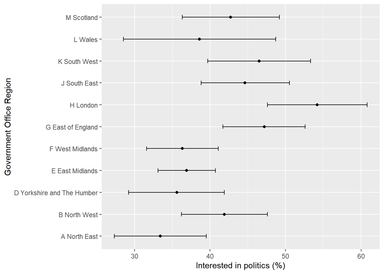
                           politics_interest ci_l ci_u
A North East                            33.4 27.3 39.5
B North West                            41.9 36.2 47.6
D Yorkshire and The Humber              35.6 29.2 41.9
E East Midlands                         36.9 33.1 40.7
F West Midlands                         36.3 31.6 41.1
G East of England                       47.2 41.7 52.6
H London                                54.2 47.6 60.8
J South East                            44.6 38.8 50.5
K South West                            46.5 39.7 53.3
L Wales                                 38.6 28.5 48.7
M Scotland                              42.7 36.3 49.2
Let’s now plot the point estimates and their confidence intervals.
The estimates show political interest varies across regions, ranging from around one-third of adults in the North East to just over one-half in London. The confidence intervals indicate that some of this variation may reflect sampling uncertainty.
8.1 An additional note on subsetting
Another way to estimate statistics for a subgroup is to analyse only respondents belonging to that group. For example, if we were interested only in respondents who are employed, we could create a subset and calculate estimates for that subgroup.
There are a few points to note when subsetting survey data.
Survey weights are usually designed to make the full sample representative of the target population. If we analyse only a subset of respondents, the weights may not necessarily produce estimates that are representative of the corresponding population subgroup.
It is important to retain all the survey design information when estimating standard errors and confidence intervals. If subsetting, you should create the survey design object first and then subset using the subset() function. This ensures that the survey weights, clustering and stratification information are retained in the analysis.
Although subsetting can be useful when analysing a subgroup, domain estimation using svyby() is generally the preferred approach because it is simpler, less prone to error and naturally retains the survey design information.
8.2 Key points
Domain estimates describe subgroups of the population, such as regions, age groups or men and women.
svyby() can be used to estimate statistics for multiple subgroups in a single command while accounting for the survey design.
If new variables are added to the dataset after creating a survey design object, the survey design object should be recreated before analysis.
Be cautious when analysing a subgroup separately. Survey weights may not make the subsample representative of the corresponding population subgroup. Always create the survey design object first and then use subset() to retain all the survey design information.