Since the FRS data are collected at different levels—households, families (benefit units), and individuals (persons)—and provided in multiple files, you may at some point want to conduct analysis across different levels. Some files focus on specialised topics such as assets, childcare, mortgages, and pensions, which may require exploring associations between variables entered in separate files.
For example, what if we want to examine how pension type varies across genders?
In that case, it is necessary to combine data, as the two variables of interest are entered in different FRS datasets.
In this exercise, we will show how to merge data from the 2022–2023 Family Resources Survey (FRS) to explore the association between variables available in various FRS datasets. We will also assess the effect of survey weights on the results using SPSS.
Getting started
1. The dataset
The dataset we will be using in this exercise is the Family Resources Survey, 2022-2023. These data are safeguarded. You can download them from the UK Data Service after registration.
To get the Family Resources Survey (FRS), 2022-2023 dataset, go to the data catalogue page, login to your account (create an account if you do not already have one), download and save the SPSS version, which we will use in this exercise.
Create a new folder to save the downloaded data and analysis work in appropriate location on your machine and give that folder a name.
The exercise below assumes that the dataset has been saved in a new folder named UKDS on your Desktop (Windows computers). The path would typically be C:\\Users\\YOUR_USER_NAME\\Desktop\\UKDS. You can change it to the location that best suits you.
Remember to adjust the code below to match the location of the data on your machine.
The FRS is a hierarchical dataset provided every year in multiple data files (known as ‘tables’ in the FRS language). The number of these tables varies, depending on the year of the survey. The 2022-2023 FRS has 25 tables. In this exercise, we will use the general-purpose table “adult.sav” and the specialised table “pension.sav” to:
- Merge datasets to explore the association between variables available in different FRS tables.
- Apply the survey weights and compare unweighted and weighted frequencies and percentages.
2. Setting up SPSS
Setting up and showing the working directory
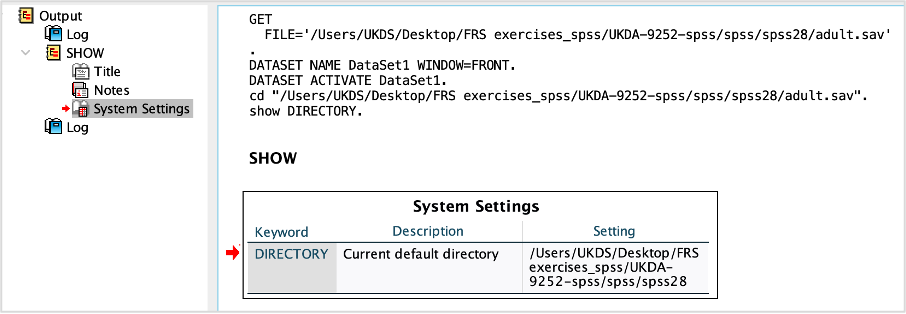
First, define the location of the working directory at the beginning of your SPSS syntax file. You can do this using thecd command, which stands for “change directory”.
You can check the working directory using the show DIRECTORY command.
cd 'C:\Users\YOUR_USER_NAME\Desktop\UKDS'.
show DIRECTORY.Note: change the command above to match your working directory.
Opening the two FRS tables in SPSS format in R
We start by opening the four datasets adult.sav and pension.sav that we will be using in this exercise. If you have your working directory saved to the folder location, the following code should open these datasets:
GET FILE='UKDA-9252-spss/spss/spss28/adult.sav'.
GET FILE='UKDA-9252-spss/spss/spss28/pension.sav'.
3. Preparing the datasets
After opening the FRS tables, we begin with exploring the adult.sav and pension.sav datasets.
But first, we will have a quick look at the number of observations (cases) and the number of the variables in these tables. You can do this by either inspect variables and cases in the Data view or use the codes below to produce a summary of all the variables in each dataset. We will start with the adult.sav dataset as follows:
GET FILE='UKDA-9252-spss/spss/spss28/adult.sav'.
  CODEBOOK all.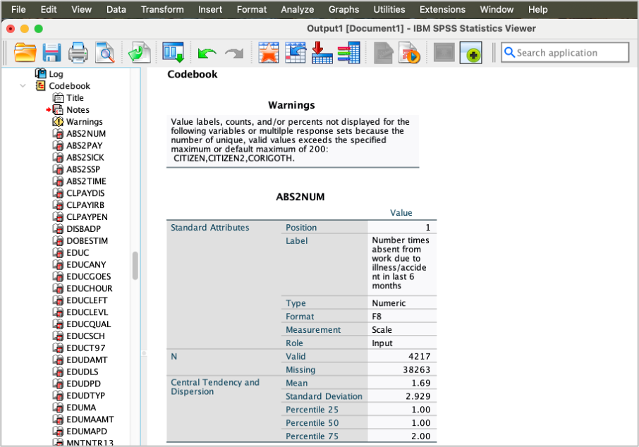
You can repeat the same steps to get a summary of all the variables in pension.sav dataset as follows:
GET FILE='UKDA-9252-spss/spss/spss28/pension.sav'.
  CODEBOOK all.
You can see that frs_adult2223 table has 587 variables. The specialised table frs_pension2223 has less variables (50 variables).
4. The variables
In this exercise, we will use only a few variables from each table. Therefore, we will create subset datasets from these two tables, containing the variables needed for the exercise. The tables below display the selected variables (names and labels) from each table.
| Variable name | Variable label |
|---|---|
| Variables from the frs_adult2223 table | |
| SERNUM | Sernum |
| BENUNIT | Benefit Unit |
| PERSON | Person |
| HEALTH1 | Whether has a long standing illness |
| SEX | Sex |
| IAGEGR4 | Individual Adult 5 Year Age Bands - Anon |
| GROSS4 | Grossing variable |
| Variables from the frs_pension2223 table | |
| SERNUM | Sernum |
| BENUNIT | Benefit Unit |
| PERSON | Person |
| PENPAY | Amount of last payment from pension (continuous variable) |
| PENTYPE | Pension Type |
#Create subset datasets from the original data files
#Use match files and Keep commands
#The code below just keeps the variables we are interested in. We will name the new datasets as frs_adult2223_short and frs_pension2223.

GET FILE='UKDA-9252-spss/spss/spss28/adult.sav'.
match files FILE = */keep SERNUM, BENUNIT, PERSON, GROSS4, HEALTH1, SEX, IAGEGR4
Save OUTFILE='frs_adult2223_short.sav'
/COMPRESSED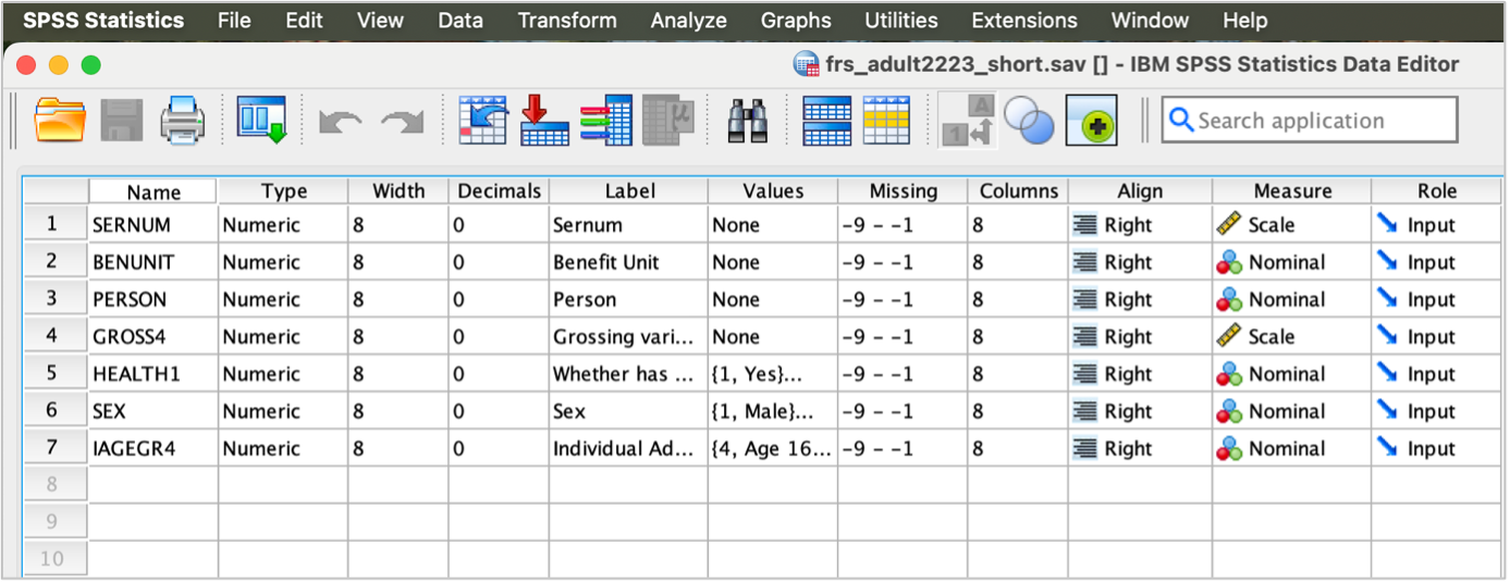
GET FILE='UKDA-9252-spss/spss/spss28/pension.sav'.
match files FILE = */keep SERNUM, BENUNIT, PERSON, PENPAY, PENTYPE
Save OUTFILE='frs_pension2223_short.sav'
/COMPRESSED 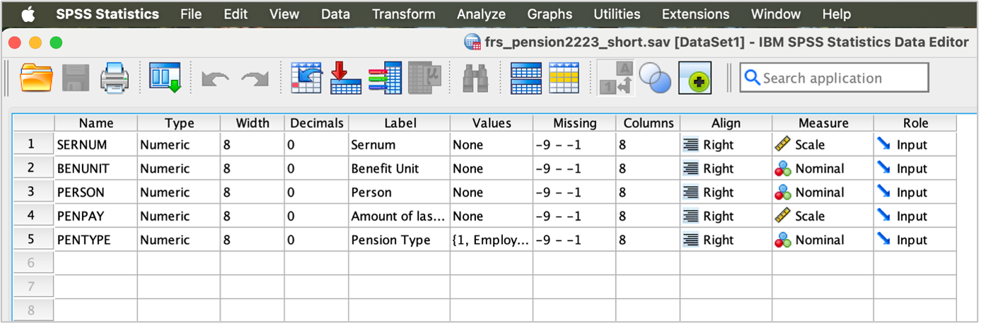
Explore the datasets
If you want to learn more about the two newly generated datasets frs_adult2223_short and frs_pension2223_short, as well as the variables we will use in this exercise, see “Explore the datasets” and “Examining the variables” sections in Exercise 1 : Using SPSS.
Merging datasets
To merge data, you need to use a common identifier - unique keys present across all datasets involved in the merge.
The Background Information and Methodology document within the FRS 2022-23 documentation provides us with the necessary information: what are the available identifiers and how to use them depending on which datasets we want to merge.
In our case, we will use the SERNUM, BENUNIT and PERSON variables to merge the two datasets: frs_adult2223_short and frs_pension2223_short. Sernum represents the unique serial number of the household, Benunit represents the identifier for the benefit unit (family) in the household, and PERSON represents the identifier for the individual. These variables are available in the two datasets we want to merge.
Merging data in SPSS
There are several types of data merge in SPSS (one-to-one, one-to-many or many-to-one). So, when merging two datasets using three key variables, the number of observations in the merged dataset depends on the type of merge and the matching criteria based on the three key variables. For successful merge, make sure both datasets are sorted by the key variables before merging. If duplicates exist in one or both datasets for the key variables, SPSS will produce all combinations of matching rows. Therefore, it is important to handle any duplicates before merging datasets.
In this example, we will use one-to-many merge. So, we expect that the number of observations in the merged dataset will be equal to the number of observations in the smaller dataset that have all three key variables in the larger dataset. The exact number of observations in the merged dataset depends on how many of the three key variables match between the two datasets.
The two variables we are focusing on: SEX, which measures gender is in frs_adult2223_short, and PENTYPE, which measures Pension Type is in frs_pension2223_short.
To merge frs_adult2223_short and frs_pension2223_short datasets, we use the following code (we will name the new data merged_data):
GET FILE='UKDA-9252-spss/spss/frs_pension2223_short.sav'.
SORT CASES BY SERNUM BENUNIT PERSON.

GET FILE='UKDA-9252-spss/spss/frs_adult2223_short.sav'.
SORT CASES BY SERNUM BENUNIT PERSON.

GET FILE='UKDA-9252-spss/spss/frs_pension2223_short.sav'.
MATCH FILES /FILE=*
  /TABLE='UKDA-9252-spss/spss/frs_adult2223_short.sav'
  /BY SERNUM BENUNIT PERSON.
EXECUTE.

Save OUTFILE="merged_data.sav"
/COMPRESSED- How many observations in the new merged_data dataset?
- How many variables in the new merged_data dataset?
- Did you expect that outcome?
- There are 15233 observations in the new merged_data as in frs_pension2223_short dataset.
- There are 9 variables in the new merged_data, which are the total number of variables in frs_adult2223_short and frs_pension2223_short datasets.
- This outcome is expected because the new merged data will include all the matched observations (rows) based on the total number of unique key combinations in both datasets. In this case, the three unique keys we used from both datasets SERNUM, BENUNIT and PERSON matched 15233 observations between the two datasets frs_adult2223_short and frs_pension2223_short, which are all the observations in frs_pension2223_short dataset (the smaller dataset). Also, the number of variables in the new merged_data (9 variables) represents the total number of variables in frs_adult2223_short and frs_pension2223_short datasets.
Before we assess the association between PENTYPE and SEX, let’s check the frequencies of the two variables after merging the two datasets frs_adult2223_short and frs_pension2223_short.
GET FILE='UKDA-9252-spss/spss/merged_data.sav.
FREQUENCIES VARIABLES=SEX PENTYPE
  /ORDER=ANALYSIS.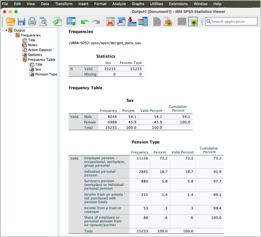
To assess the association between pension type PENTYPE and gender SEX (how pension type varies by gender), we use the following code:
GET FILE='UKDA-9252-spss/spss/merged_data.sav'.
CROSSTABS
  /TABLES=PENTYPE BY SEX
  /FORMAT=AVALUE TABLES
  /CELLS=COUNT COLUMN
  /COUNT ROUND CELL.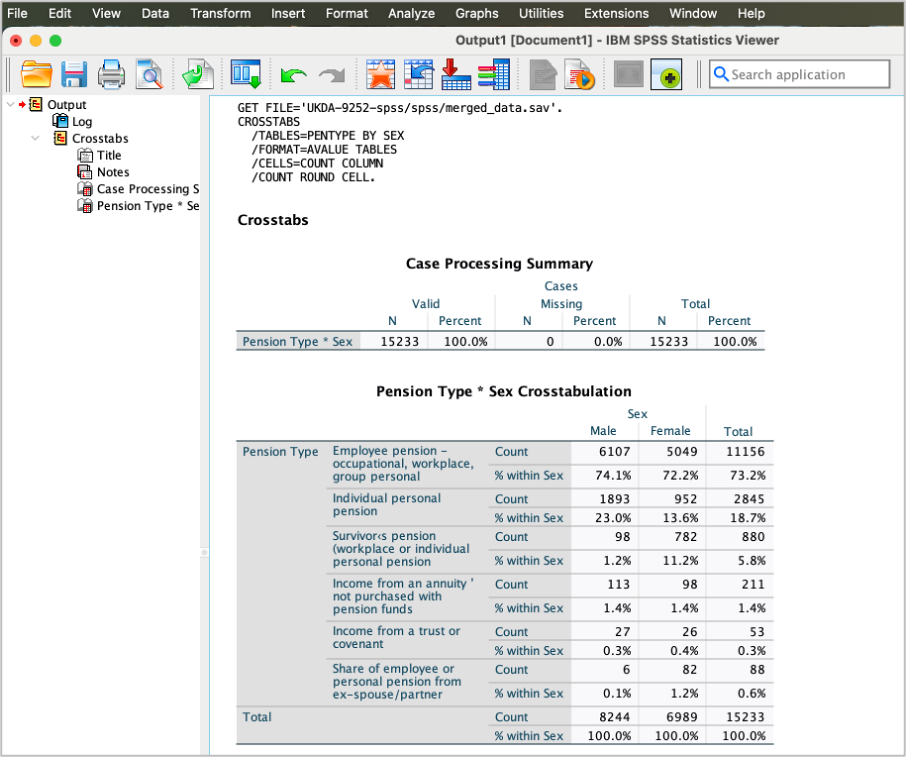
- Which type of pension was the least common for men and women?
- ‘Share of employee or personal pension from ex-spouse/partner’ was the least common pension type for men. ‘Income from a trust or covenant’ was the least common pension type for women.
Applying the weight
Now, we will apply the WEIGHT command to create weighted frequencies and percentages for the variable PENTYPE. We will then compare the results with the unweighted analyses.
Note: some weighting methods interpret weighted counts as sample sizes, leading to inaccurate standard errors and confidence intervals, particularly when weights scale to the population size. This affects standard SPSS weighting procedures, so for accurate standard errors with FRS, the Complex Samples commands should be used (available in SPSS Premium or as an add-on). However, the standard SPSS weighting commands can still calculate estimates such as means, proportions, or weighted frequencies, as shown in the example below.
PENTYPE (weighted frequency table)
- We first apply the weight GROSS4 on cases using the code below:
GET FILE='UKDA-9252-spss/spss/merged_data.sav'.
WEIGHT BY GROSS4.- To create the weighted frequency table for the PENTYPE variable, use:
GET FILE='UKDA-9252-spss/spss/merged_data.sav'.

FREQUENCIES VARIABLES=PENTYPE
  /ORDER=ANALYSIS.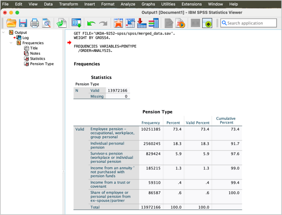
PENTYPE (weighted frequency table)
- Now we run unweighted frequencies and percentages for the PENTYPE variable to compare with the weighted frequencies and percentages.
Stop weighting the data using WEIGHT off command, then get a frequency table for the PENTYPE variable.
WEIGHT OFF.
GET FILE='UKDA-9252-spss/spss/merged_data.sav'.
FREQUENCIES VARIABLES=PENTYPE
  /ORDER=ANALYSIS.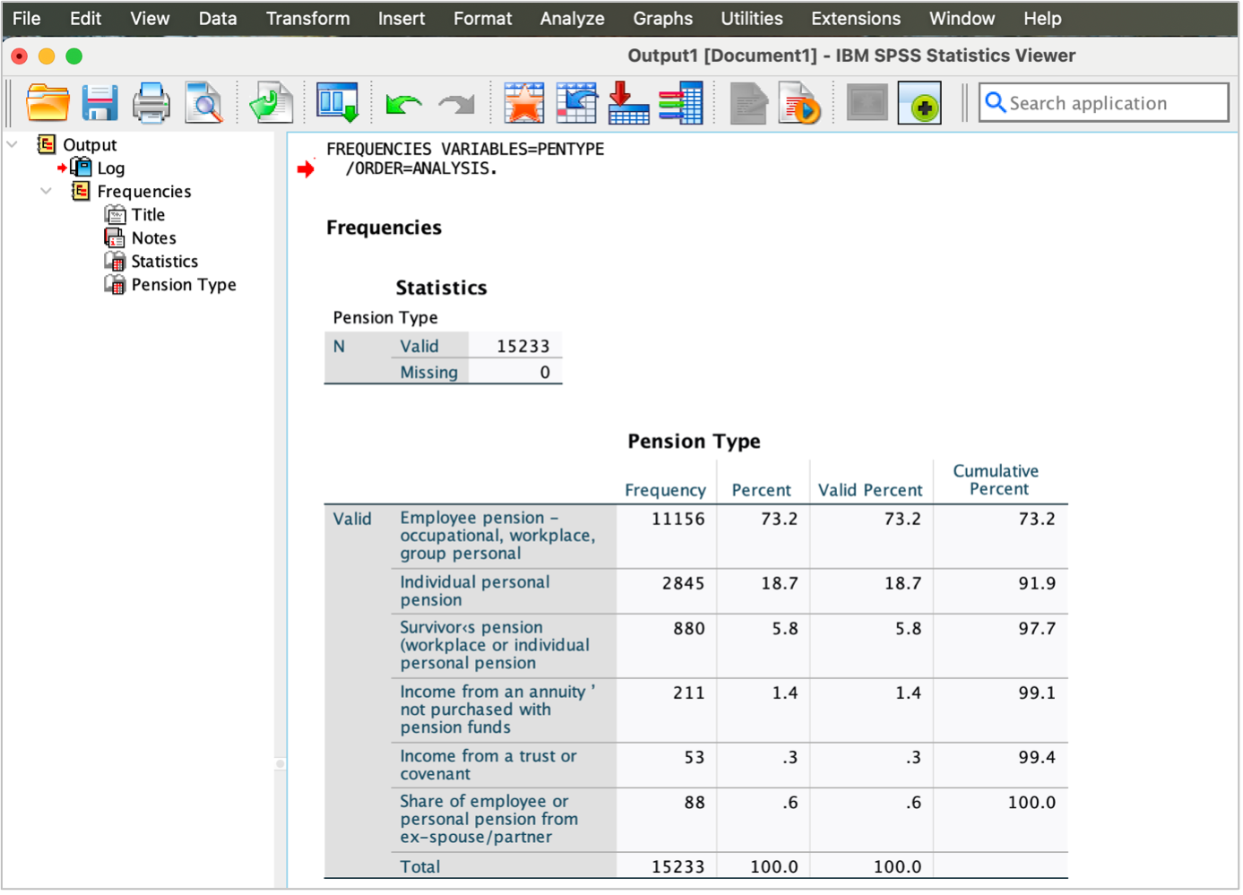
- Do the frequencies change when the weight is applied?
- Are there differences between the percentages of PENTYPE for the weighted and unweighted analyses?
- Yes, the frequencies change substantially; the frequencies are much higher when the weight is applied. The large change is because the weights in the FRS sum to known population totals, which helps population totals to be estimated easily.
The weights in the FRS also ensure that estimates reflect the sample design so that cases with a lower probability of selection will receive a higher weight to compensate for differential non-response among different subgroups in the population, and as such should help guard against potential non-response bias.
- We summarise the weighed and unweighted percentages of PENTYPE in the table below to make the comparison easier:
| PENTYPE | Weighted (%) | Unweighted (%) |
|---|---|---|
| Employee pension - occupational, workplace, group personal | 73.37 | 73.24 |
| Individual personal pension | 18.32 | 18.68 |
| Survivor‹s pension (workplace or individual personal pension | 5.94 | 5.78 |
| Income from an annuity ’ not purchased with pension funds | 1.33 | 1.39 |
| Income from a trust or covenant | 0.42 | 0.35 |
| Share of employee or personal pension from ex-spouse/partner | 0.62 | 0.58 |
You can see that there are very small differences between the percentages of PENTYPE for the weighted and unweighted analyses. However, that is not always the case. You should always apply weights when you conduct data analysis.
Your turn!
Carry out a weighted and unweighted analysis to assess the frequencies and percentages of the gender variable in the merged_data (use the variable: SEX).
Outcome!
Weighted SEX
GET FILE='UKDA-9252-spss/spss/merged_data.sav'.
WEIGHT BY GROSS4.

FREQUENCIES VARIABLES=SEX
  /ORDER=ANALYSIS.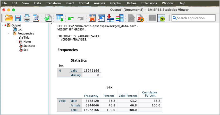
Unweighted SEX
WEIGHT OFF.
GET FILE='UKDA-9252-spss/spss/merged_data.sav'.
FREQUENCIES VARIABLES=SEX
  /ORDER=ANALYSIS.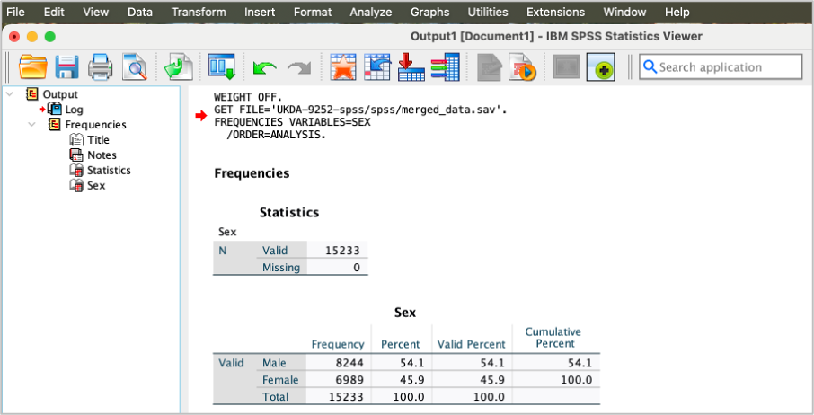
We summarise the weighed and unweighted percentages of SEX in the table below to make the comparison easier:
| SEX | Weighted (%) | Unweighted (%) |
|---|---|---|
| Male | 53.16 | 54.12 |
| Female | 46.84 | 45.88 |
There are noticeable changes in the frequencies of SEX when the weight is applied (they are much higher). But the differences between the percentages for the weighted and unweighted analysis are small.